>	restart; with(plots): with(VectorCalculus):

 

Warning, the name changecoords has been redefined 

Warning, the assigned names `<,>` and `<|>` now have a global binding 

Warning, these protected names have been redefined and unprotected: `*`, `+`, `-`, `.`, D, Vector, diff, int, limit, series 

rB and rL are radial parameters that determine how "big" and "fat" the 

torus is. rB is the distance from the "center" of the torus to the circle 

lying in the "center" of the ring. rL is the radius of the "ring" itself. 

m determines how many times the curve is to wrap around the torus. 

>	rB := 4; rL := 1; m := 4;

 

>	xc := (phi,theta,r) -> (r*cos(phi)+rB)*cos(theta); yc := (phi,theta,r) -> (r*cos(phi)+rB)*sin(theta); zc := (phi,theta,r) -> r*sin(phi);

 

We should make the torus that the curve wraps around slightly smaller than the 

curve -- so the curve is on the "outside" of the torus. 

>	sc := 0.95;

 

>	torusEqn := (sqrt(x^2+y^2)-rB)^2+z^2 = (sc*rL)^2;

 

>

t1 := plot3d([xc(phi,theta,sc*rL),yc(phi,theta,sc*rL),zc(phi,theta,sc*rL)],             phi=0..2*Pi,theta=0..2*Pi,color=grey,scaling=constrained); c1 := spacecurve([xc(m*theta,theta,rL),yc(m*theta,theta,rL),zc(m*theta,theta,rL)],             theta=0..2*Pi,color=blue,scaling=constrained,numpoints=5000,thickness=3);

 

>	display3d(t1,c1);

 

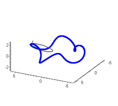
Here we construct the osculating circle (oscCt gives parametric equations at time t). 

>	r := t -> < xc(m*t,t,rL), yc(m*t,t,rL), zc(m*t,t,rL) >;

 

>	tnbFrame := TNBFrame(r(t),t): kappa := Curvature(r(t),t):

 

>	Tt := tnbFrame[1]: Nt := tnbFrame[2]: Bt := tnbFrame[3]:

 

>	oscCt := (cos(theta)/kappa)*Tt+(sin(theta)/kappa)*Nt+(1/kappa)*Nt+r(t):

 

k_0 is the number of frames to generate for the animation. 

NOTE: It may take a while to generate hundreds of frames. 

To animate without displaying the torus, remove "t1" from 

the "myAnimL ... display3d({....}...);" command below. 

>	k[0] := 150;

 

>

myAnimL := array(1..k[0]+1): for t[0] from 0 by 1 to k[0] do   PoscC := spacecurve(subs(t=(2*Pi/k[0])*t[0],oscCt),theta=0..2*Pi,                       color=black,thickness=2,scaling=constrained):   PTt := arrow(subs(t=(2*Pi/k[0])*t[0],r(t)),subs(t=(2*Pi/k[0])*t[0],Tt),                color=red,thickness=2):   PNt := arrow(subs(t=(2*Pi/k[0])*t[0],r(t)),subs(t=(2*Pi/k[0])*t[0],Nt),                color=yellow,thickness=2):   PBt := arrow(subs(t=(2*Pi/k[0])*t[0],r(t)),subs(t=(2*Pi/k[0])*t[0],Bt),                color=green,thickness=2):   myAnimL[t[0]+1] := display3d({t1,c1,PoscC,PTt,PNt,PBt},scaling=constrained): end do:

 

>	display(seq(myAnimL[i],i=1..k[0]),insequence=true,scaling=constrained);

 

>

myAnimL2 := array(1..k[0]+1): for t[0] from 0 by 1 to k[0] do   PoscC := spacecurve(subs(t=(2*Pi/k[0])*t[0],oscCt),theta=0..2*Pi,                       color=black,thickness=2,scaling=constrained):   PTt := arrow(subs(t=(2*Pi/k[0])*t[0],r(t)),subs(t=(2*Pi/k[0])*t[0],Tt),                color=red,thickness=2):   PNt := arrow(subs(t=(2*Pi/k[0])*t[0],r(t)),subs(t=(2*Pi/k[0])*t[0],Nt),                color=yellow,thickness=2):   PBt := arrow(subs(t=(2*Pi/k[0])*t[0],r(t)),subs(t=(2*Pi/k[0])*t[0],Bt),                color=green,thickness=2):   myAnimL2[t[0]+1] := display3d({t1,c1,PoscC,PTt,PNt,PBt},scaling=constrained,                                 orientation=[45,-90*(sin((t[0]*Pi)/k[0]))+45]): end do:

 

>	display(seq(myAnimL2[i],i=1..k[0]),insequence=true,scaling=constrained);