math5230-fall2016-visualizing

Visualizing Determinants (Linear Algebra)

> restart;
with(plottools):
with(plots):
with(LinearAlgebra):

> # Template list (Converting from a matrix to the vertices of a parallelogram.)
listA := [[0,0],[A[1,1],A[1,2]],[A[1,1]+A[2,1],A[1,2]+A[2,2]],[A[2,1],A[2,2]]];

(1)

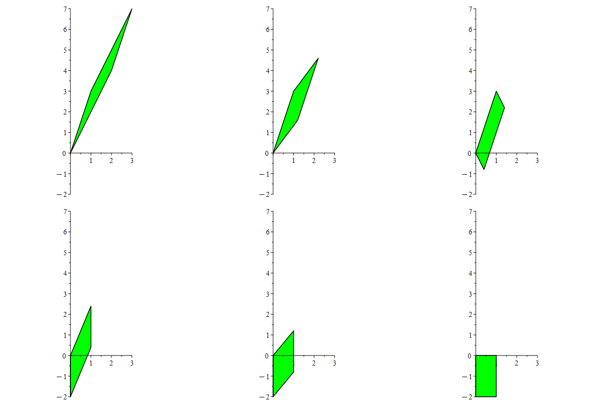
Each "for" loop performs type III operations in such a way that a target entry is cleared little-by-little. First, the (2,1)-entry "2" is cleared. Then the (1,2)-entry "3" is cleared. This leaves us with a diagonal matrix (whose plot is a rectangle).

Type III operations shear our parallelogram. These operations don't change the area. In this way we can see why the determinant (which is unchanged by type III operations) computes areas/volumes.

> A := <<1,2>|<3,4>>:

Area = abs(Determinant(A));

B := A;

for i from 0 to 10 do
  A := RowOperation(B,[2,1],-2*(i/10));
  showA[i] := polygon(listA);
end do:

B := RowOperation(B,[2,1],-2,inplace=true);

for i from 0 to 10 do
  A := RowOperation(B,[1,2],3/2*(i/10));
  showA[i+11] := polygon(listA);
end do:

B := RowOperation(B,[1,2],3/2,inplace=true);

Typesetting:-mfenced(Typesetting:-mrow(Typesetting:-mtable(Typesetting:-mtr(Typesetting:-mtd(Typesetting:-mn(

(2)

> display(seq(showA[i],i=0..21),color=green,insequence=true,scaling=constrained);

Plot_2d

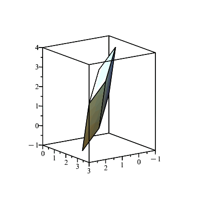
Let's do the same thing with a 3x3 matrix (i.e. a parallelepiped).

> A := 'A';
listA := seq([seq(A[i,j],j=1..3)],i=1..3);

(3)

> A := <<1,2,-1>|<2,2,0>|<3,-1,1>>;
display(parallelepiped(listA),scaling=constrained);

Typesetting:-mfenced(Typesetting:-mrow(Typesetting:-mtable(Typesetting:-mtr(Typesetting:-mtd(Typesetting:-mn(

Plot_2d

> A := <<1,2,-1>|<2,2,0>|<3,-1,1>>:

Volume = abs(Determinant(A));

B := A;

for i from 0 to 10 do
  A := RowOperation(B,[2,1],-2*(i/10));
  showA[i] := parallelepiped(listA);
end do:

B := RowOperation(B,[2,1],-2,inplace=true);

for i from 0 to 10 do
  A := RowOperation(B,[3,1],1*(i/10));
  showA[i+11] := parallelepiped(listA);
end do:

B := RowOperation(B,[3,1],1,inplace=true);

for i from 0 to 10 do
  A := RowOperation(B,[3,2],1*(i/10));
  showA[i+22] := parallelepiped(listA);

end do:

B := RowOperation(B,[3,2],1,inplace=true);

for i from 0 to 10 do
  A := RowOperation(B,[2,3],-7/3*(i/10));
  showA[i+33] := parallelepiped(listA);
end do:

B := RowOperation(B,[2,3],-7/3,inplace=true);

for i from 0 to 10 do
  A := RowOperation(B,[1,3],1*(i/10));
  showA[i+44] := parallelepiped(listA);
end do:

B := RowOperation(B,[1,3],1,inplace=true);

for i from 0 to 10 do
  A := RowOperation(B,[1,2],1*(i/10));
  showA[i+55] := parallelepiped(listA);
end do:

B := RowOperation(B,[1,2],1,inplace=true);

Typesetting:-mfenced(Typesetting:-mrow(Typesetting:-mtable(Typesetting:-mtr(Typesetting:-mtd(Typesetting:-mn(

(4)

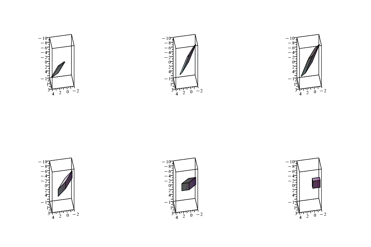
Again, the volume is unchanged as we shear (i.e., do Type III operations). However, due to our viewing angle, at times is seems that the volume changes (but it doesn't).

> display(seq(showA[i],i=0..65),insequence=true,scaling=constrained,orientation=[190,220]);

Plot_2d