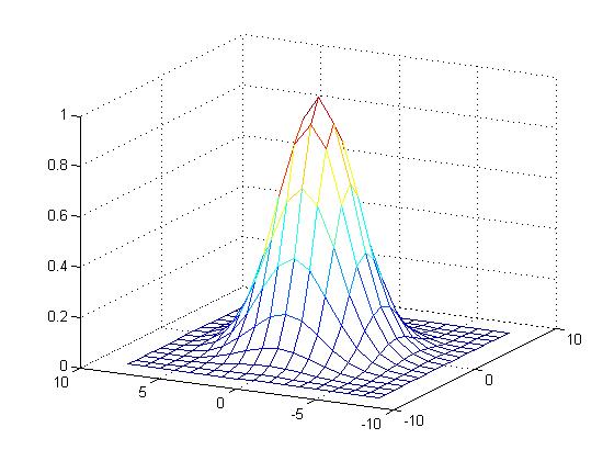
[> GuassianPSF(0.1,0);
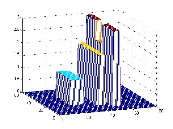
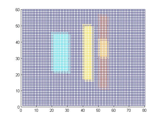
[> A = cityScape(0);
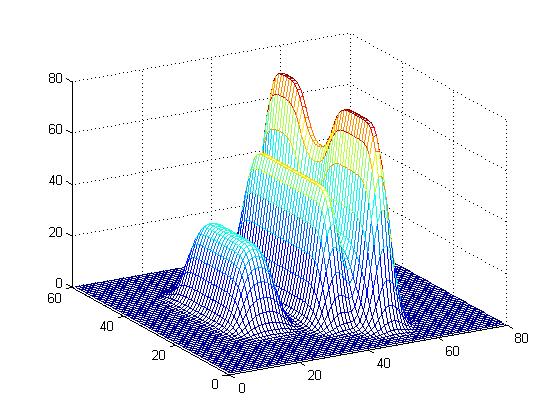
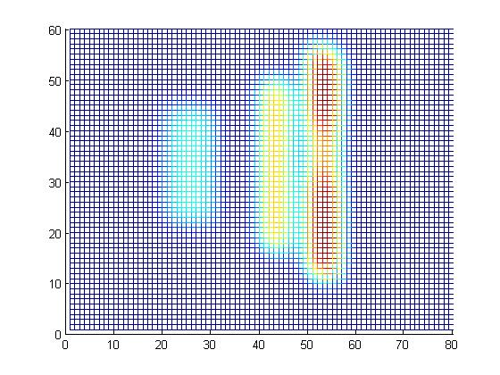
[> applyGaussianPSF(0.1, A, 0);
An image can be thought of as an array filled with numbers. Grayscale images can be stored as \( m \times n \) matrices whose entries determine the shade of gray. Color images can be stored as \( m \times n \times 3 \) tensors (think 3 matrices stacked on top of each other). Each level keeps track of the shade of Red, Green, or Blue (RGB values).
To apply methods from linear algebra it is helpful to think of images as vectors (\(m \times 1\) arrays). To convert from a rectangular array to a matrix we simply rip out all of the columns and then stack them end to end.
\( \begin{vmatrix} 1 & 2 & 3 \\ 1 & 0 & 2 \end{vmatrix} \quad \Longrightarrow \quad \begin{array}{c} \begin{vmatrix} 1 \\ 1 \end{vmatrix} \\ \; \\ \begin{vmatrix} 2 \\ 0 \end{vmatrix} \\ \; \\ \begin{vmatrix} 3 \\ 2 \end{vmatrix} \end{array} \quad \Longrightarrow \quad \begin{vmatrix} 1 \\ 1 \\ 2 \\ 0 \\ 3 \\ 2 \end{vmatrix} \)An image is blurring when the pixels making up the image are "smeared" and spread around. We spread out pixels using a point spread function (PSF). In particular we used a Gaussian PSF (sort of like a 3D bell curve).
|
[> GuassianPSF(0.1,0); |
|
[> A = cityScape(0); |
|
[> applyGaussianPSF(0.1, A, 0); |
The PSF is applied to each pixel then these smears are added together. Since this is a "linear" process it amounts to multiplying our image vector by a matrix. So if \( x \) is our unblurred image and \( A \) is the matrix corresponding to the PSF blurring process, then the blurred image is \( Ax = b \).
Now given a blurred image \( b \) we "simply" need to solve the system \( Ax=b \) for \( x \). In linear algebra we learn to solve linear systems using "row reduction". It turns out that this won't work for us for sveral reasons.
Our way around the first two difficulties (round-off error & large coefficient matrix) is to use an "iterative" method to solve the system. This type of method takes in a "guess" solution and then (hopefully) improves the guess. This improved guess is then fed back into the method to improve it yet again, etc. Iterative methods have the avantage that then don't require us to manipulate the coefficient matrix (\( A \)). In fact, in our code we don't ever construct the matrix \( A \) itself -- we instead have a function "applyGaussianPSF" which mimics the effect of multiplying by \( A \). This saves us from having to store the potentially millions or billions of entries of \( A \).
The particular interative method we chose is called the "Conjugate Gradient Method"
(CG method). The CG method is based on a process of "sliding down hill". Consider the
following complicated looking function:
\( f(x) = \frac{1}{2}x^T A x - x^T b \)
The graph of \( f \) is some sort of "hyper-surface". In Calculus III one learns
about gradient vectors. The gradient of a function, \( \nabla f \), is a vector which
points in the direction of maximal increase. The negative of the gradient then points
in the direction of maximal decrease. It turns out that the gradient of \( f \) is
\( \nabla f = Ax-b \)
Therefore, \( \qquad \nabla f = 0 \qquad \Longleftrightarrow \qquad Ax-b = 0
\qquad \Longleftrightarrow \qquad Ax=b \)
Points where the gradient vector are zero are critical points. If we want to solve
our system, we need to find a "minimum" for \( f \). We can do this by picking some
point on our surface and then heading down hill. To get to the minimum as fast
as possible we should head down hill along \( - \nabla f \) since that is the direction
of maximal decrease. That is basically what the CG method does.